Support:UniSA
From Headus Docs
| Revision as of 03:56, 30 July 2010 (edit) Headus (Talk | contribs) ← Previous diff |
Current revision (08:16, 23 July 2014) (edit) (undo) Headus (Talk | contribs) (→Bounding Measure Method) |
||
| (23 intermediate revisions not shown.) | |||
| Line 18: | Line 18: | ||
| "Place Landmarks" tool to quickly place points on all of your color markers. | "Place Landmarks" tool to quickly place points on all of your color markers. | ||
| + | <!-- | ||
| === Wish/Bug List === | === Wish/Bug List === | ||
| - | "I’m going to upload a BAF.ply file + its slice and a txt file of our measure list. Our problems now is that when we re-open the baf and restore our measurements, some of these (points and measures) are in different places, missed or even we have new curves… Also, the new function to look for max and min girths changes its spot after restoring." | + | * one file missing slice through head after merging |
| - | "In addition, just in case Mike didn’t mention it to you, we are having problems when we want to find the max hip girth when using a curve guide, since the curve doesn’t always go all the way around – sometimes it’s missing part of the girth." | + | * when we re-open the baf and restore our measurements, some of these (points and measures) are in different places, missed or even we have new curves… |
| - | "Lastly, we found that when we want to export the tape value we have to pick each line and press the key “T” before exporting. Is this the only way to do it or we are missing some quicker way of toggling all tape measures at once." | + | * the new function to look for max and min girths changes its spot after restoring. |
| - | "but if CySize could automatically generate a straight but inclined line between the two armpit markers, that would be great." | + | * it would be beneficial to temporarily or permanently remove markers |
| - | "clip the raised landmarks off and if so, can we clip them individually? Sometimes it would be beneficial to temporarily or permanently remove markers" | + | * <strike> generate a straight but inclined line between the two armpit markers, </strike> |
| + | |||
| + | * <strike> Crashes when use Shift-T to tape measure all curves. </strike> | ||
| + | --> | ||
| + | <!-- | ||
| + | === Upload folder for Windows XP === | ||
| + | |||
| + | These instructions apply to Windows XP, but should be OK for other Windows versions: | ||
| + | |||
| + | # Open the 'My Network Places' folder. If you don't know where this is, go to 'Start -> Help' and search for 'add network place', then look for a 'My Network Places' link in the help documentation. | ||
| + | # Once you have the 'My Network Places' folder open, double click 'Add a network place.' | ||
| + | # When asked where you want to create the network place, select 'Choose another network location' | ||
| + | # In the 'Type the location of the Network Place' text box, enter in '''<nowiki>http://www.headus.com:80/au/clients/unisa/upload</nowiki>''' | ||
| + | # Enter '''unisa''' for the User name, and '''olds''' for the Password | ||
| + | # In the 'Enter a name for this Network Place' text box, enter "headus Upload". | ||
| + | # To complete the setup, click Finish. A Microsoft Web Folder appears showing the contents of the upload folder. | ||
| + | |||
| + | To upload files, just drag'n'drop them into this folder. | ||
| + | |||
| + | You may see two files in this directory - .htaccess and .htpasswd - when you connect to it. These files do need to be there and you won't be able to delete them, so they can safely be ignored. | ||
| + | --> | ||
| + | |||
| + | === Bounding Measure Method === | ||
| + | |||
| + | <table><tr><td> | ||
| + | |||
| + | {{img|UniSA-bound10.jpg|Determine Axis}} | ||
| + | |||
| + | The first step is to determine the axis of the bounding volume. Another way to look at it could be the direction of travel that the object would be moving in. | ||
| + | |||
| + | By default its the direction defined by the start and end points of of the section guide curve, and this is illustrated in the middle image in {{fig}}. The right image shows the difference in slicing direction for a Z-axis tagged section. | ||
| + | |||
| + | {{img|UniSA-bound11.jpg|Cut Sections}} | ||
| + | |||
| + | Next the mesh is sliced through, perpendicular to the bounding axis, and all these slices are then moved along the bounding axis so that they are co-planar (see {{fig}}). | ||
| + | |||
| + | {{img|UniSA-bound12.jpg|Convex Hull}} | ||
| + | |||
| + | Finally the convex hull of the gathered slices is calculated (see {{fig}}), and this profile is then projected back along the bounding axis to create the blue volume displayed in the software. | ||
| + | |||
| + | </td></tr></table> | ||
Current revision

[edit] Vitronic Color Import
To import Vitronic color scans into CySize, you need to follow these steps:
- Run PlyTool as you normally would.
- Tick the "UV to CPV" option (see Fig 1).
- Click the arrow and load the first color texture file.
- Set the rotation angles to 90, 0, 90.
- Click the Input arrow and load the OBJ file with Meters ticked (see Fig 2). Even if you already have an OBJ loaded, you need to reload it after ticking the "UV to CPV" option.
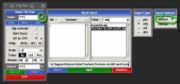 Fig 2. Load OBJ
 - Click the Output arrow and specify the PLY file as you normally would.
- Click Convert
- Click View, and use the 'C' key to shade the mesh with color to check the conversion.

Load the PLY file into CySize and process as you normally would and the color should end up in the final merged and filled surface. You can then use the "Place Landmarks" tool to quickly place points on all of your color markers.
[edit] Bounding Measure Method
 Fig 3. Determine Axis The first step is to determine the axis of the bounding volume. Another way to look at it could be the direction of travel that the object would be moving in. By default its the direction defined by the start and end points of of the section guide curve, and this is illustrated in the middle image in Fig 3. The right image shows the difference in slicing direction for a Z-axis tagged section.  Fig 4. Cut Sections Next the mesh is sliced through, perpendicular to the bounding axis, and all these slices are then moved along the bounding axis so that they are co-planar (see Fig 4).  Fig 5. Convex Hull Finally the convex hull of the gathered slices is calculated (see Fig 5), and this profile is then projected back along the bounding axis to create the blue volume displayed in the software. |